A SURVIVAL ANALYSIS APPROACH TO UNDERSTANDING TRAVEL TIME DECAY
Aaron Weinstock
November 27, 2019
1 INTRODUCTION
Historically, travel time decay curves have been estimated via exponential regression on time. First, for each time t in a set of travel times \({\scriptstyle t = 1, 2, ..., t_{max}}\), number of trips lasting at least t minutes would be calculated. Then, assuming the functional form y = \(Ae^{bt}\), a regression would be fit with t (time) as the sole explanatory variable and y (the number of trips lasting at least t minutes) as the response.
While this method does elucidate the underlying decay curve, it is a naive approach in that it assumes travel time decay relies only on time. By considering time as the only covariate, this type of model ignores the impact other variables could have on travel time decay. For example, increased age could be associated with shorter tripmaking for walking trips, and thus a steeper travel time decay. Thus, a more informative travel time decay model may seek to include the effects of both time and other relevant covariates. This would not only produce a more realistic travel time decay curve, but allow for a quantification of the relationship between included covariates and travel time decay.
This paper suggests the use of a survival analysis approach to modeling travel time decay. Survival analysis encompasses a set of statistical methods interested in modeling the time to an “event” using a set of predictor variables. It is most often seen in clinical trials, where a researcher may be interested in how long patients survive after being given a particular treatment. It can be extended to travel time decay by considering the ending of a trip as the “event” of interest. Table 1 provides the travel time decay analogs of a more common survival analysis example.
| Common survival analysis | Analogs in trip decay | |
|---|---|---|
| Observational unit | Disease patients at a hospital | Trip records |
| Event | Death | Ending of a trip |
| Predictor variables | Treatment, age, sex | Financial cost, purpose |
| Meaning of “survival” | How long the patient survives | How long the trip lasts |
2 DATA
The data comes from the Massachusetts Travel Survey (MTS), conducted by the Massachusetts Department of Transportation and published in June 2012. It was provided by the Metropolitan Area Planning Council (MAPC), which serves Boston, MA and its metropolitan region.
The data includes 190,215 trip records from 37,023 persons across 15,033 households in Massachusetts. The trip dataset includes attributes such as duration, mode, purpose, cost, destination, etc. The person dataset includes attributes such as age, education, employment status, etc. The household dataset includes size, number of workers, number of vehicles, income, location, etc.
This analysis required known values for all model variables, so some trip records were filtered out prior to model fitting based on survey responses. In addition, models were fit individually on different classes of modes, so different filtering conditions were necessary to create each model set. Table 2 details the modes used for each model, the conditions on which model variables were filtered, and the resulting number of trip records used for model fitting.
| Model | Modes | Variable | Filter condition | Total records |
|---|---|---|---|---|
| Personal vehicle | Driver or passenger of auto, truck, van, or motorcycle | Parking cost | Not “do not know” or “refused” | 112,262 |
| Toll cost | Not “do not know” or “refused” | |||
| Household size | Not “do not know” or “refused” | |||
| Trip purpose | Not “other” or “while traveling – other”; not a “loop trip” with no secondary purpose | |||
| TAZ-based measures | Not “NA” (indicating either origin or destination is not in the study area) | |||
| Non-motorized | Walk or bike | Household size | Not “do not know” or “refused” | 26,137 |
| Trip purpose | Not “other” or “while traveling – other”; not a “loop trip” with no secondary purpose | |||
| TAZ-based measures | Not “NA” (indicating either origin or destination is not in the study area) |
3 MODELING METHODS
3.1 THE COX PROPORTIONAL HAZARDS MODEL
Of particular interest for travel time decay modeling is the Cox proportional hazards model (henceforth referred to as the Cox model). The Cox model is, in essense, a multivariate regression. It attempts to model the hazard function h(t) using a set of predictor variables. The hazard function can then be used to calculate the survival function S(t), or the probability that a trip lasts longer than t. Though hazard is not a probability, it is helpful to think of hazard as the probability that a trip will end in an infinitesimally small time window \(\scriptstyle [t, t + δt]\), provided that the trip has lasted until time t. In other words, it is the instantaneous risk of a trip ending, given that it has lasted to that point. The mathematical relationship between the survival function and the hazard function is \(\scriptstyle S(t) = e^{−\int^t_0 h(y)dy}\), where \(\scriptstyle \int^t_0 h(y)dy\) is the cumulative hazard function, or the total accumulated risk up to time t. Details are left out for clarity, but this is based on the definition of h(t) as a limit of event probability as \(\scriptstyle δ → 0\).
The Cox model is multiplicative, in that it assumes a multiplicative relationship between the covariates and the hazard. It takes the following form:
\[ h(t|x_{i1}, ...x_{ip}) = h0(t) ∗ e^{β1xi1+...+βpxip} \]
Where:
- t is time,
- \(\scriptstyle h(t|xi)\) is the hazard function for trip i with covariates \(\scriptstyle xi1, ..., xip\),
- \(\scriptstyle h0(t)\) is the baseline hazard function,
- βj is the effect of the j th covariate, and
- \(\scriptstyle x_{ij}\) is the value of the \(\scriptstyle j^{th}\) covariate for the \(\scriptstyle i^{th}\) trip
An important feature of the Cox model is that the baseline hazard function is not specified. This is due to the proportional hazards assumption: the ratio of hazards between two unique observations should not rely on time. For example, if after 15 minutes, a walking trip taken by a 60 year old carries twice the risk of ending as a walking trip taken by a 20 year old, it should also carry twice the risk after 10 minutes, 30 minutes, or indeed any other time. Non-proportional hazards may be thought of as an interaction between a covariate and time. Because hazards are all proportional under the proportional hazards assumption, the baseline hazard is arbitrary.
The Cox model is “semi-parametric”, in that it requires no assumptions about the baseline hazard function. Parametric methods can be used if the baseline hazard itself is of interest, and these methods indeed rely on specifying a distribution for the baseline hazard (common selections include the Exponential, Weibull, and Lognormal distributions). Though these models have more power when this distribution is correctly specified, they are not robust to misspecifications, and thus are highly risky. For this particular application of travel time decay curves, the baseline hazard was not of particular interest, and it sufficed to assume a general decrease in trip survival with time in the absence of covariate information (as is the outcome of Cox modeling). However, it stands to reason that understanding the baseline hazard may be of interest in other travel time decay modeling applications.
3.2 SELECTION OF COVARIATES
Covariates to be considered for each mode-specific model were selected from the set of available attributes in the trip, person, and household datasets reviewed in the Data section. Importantly, only covariates that would be (1) known for a given trip/person/household in a predictive setting or (2) easy to estimate for a given trip/person/household were selected for the model. These conditions were established for easier use of final model in practice. For example, though it is easy to see how age may be a relevant predictor of travel time decay for walking trips (older people may tend to take shorter trips, for example), it is unlikely a trip taker’s age is a readily available data point in a predictive setting. Furthermore, attempts to predict age for inclusion in a final model could be complicated and add uncertainty to travel time decay estimates.
Table 3 details the candidate covariates considered for each mode-specific model.
| Model | Covariates |
|---|---|
| Personal vehicle | Parking cost |
| Toll cost | |
| Household size | |
| Trip purpose (home, work, non-work) | |
| Terminal time (by origin and destination TAZ) | |
| Non-motorized | Parking cost (by origin and destination TAZ) |
| Household size | |
| Trip purpose (home, work, non-work) | |
| Terminal time (by origin and destination TAZ) |
In all models, trip purpose was collapsed from 24 categories provided in the MTS data to three broad “purpose groups”: home, work, and non-work. Table 4 details how purposes were collapsed. “Loop trips” were classified according to their secondary purpose (which were also coded according to Table 4), or filtered out if no secondary purpose was provided.
| Model | MAPC survey code | MAPC purpose definition |
|---|---|---|
| Home | 1 | Working at home |
| 2 | All other home activities | |
| Work | 3 | Work/job |
| 4 | All other activities at work | |
| 12 | Work business related | |
| Non-work | 5 | Volunteer work/activities |
| 6 | Attending class | |
| 7 | All other school activities | |
| 8 | Changed type of transportation | |
| 9 | Drop off passenger from car | |
| 10 | Pick up passenger from car | |
| 13 | Service private vehicle | |
| 14 | Routine shopping | |
| 15 | Shopping for major purchases | |
| 16 | Household errands | |
| 17 | Personal business | |
| 18 | Eat meal outside of home | |
| 19 | Health care | |
| 20 | Civic/religious activities | |
| 21 | Outdoor recreation/entertainment | |
| 22 | Indoor recreation/entertainment | |
| 23 | Visit friends/relatives |
3.3 INITIAL MODELS
Initial model fitting began by including all candidate covariates for each mode-specific model a linear form (see Table 3). Backward selection was applied to create a “statistically valid” model – one with only significant covariates. Backward selection involves iteratively eliminating the least significant covariate from the model [from the set of insignificant covarites], and refitting the model until all remaining covariates are significant. If all variables were significant in the first model fit, backwards selection was not applied, as there was no need for it.
3.4 THE PROPORTIONAL HAZARDS ASSUMPTION
Though there are multiple assumptions underlying the Cox model, by far the most important assumption is that of proportional hazards (see Section 3.1, The Cox proportional hazards model). Without this assumption, the Cox model is uninterpretable and completely invalid. Exploration of model diagnostics thus began with the proportional hazards assumption, and proceeded to other assumptions only once proportional hazards was verified.
The proportional hazards assumption was tested for each covariate using the Schoenfeld Residuals Test (also known as the Schoenfeld Individual Test). The null hypothesis of this test is that time and scaled Schoenfeld residuals are uncorrelated, which should be true in the case of proportional hazards. The alternative hypothesis is that time and scaled Schoenfeld residuals are correlated. Thus, a significant result indicates that a lack of proportional hazards - this would indicate the model results are dependent on time. If no time dependence was observed in any covariate at α = 0.05, diagnostics proceeded to validation of other assumptions. Otherwise, a new model accounting for time dependence was fit.
3.4.1 TIME- DEPENDENT MODELS
Multiple strategies exist to account for time dependence in Cox models. One such method is the use of “time-dependent coefficients”, which involves unique effect sizes for covariates depending on the period of time. Essentially, time-dependent coefficients create a step function of survival time, where each covariate is time-independent within each step. This is particularly relevant and interpretable in the context of travel time decay, be ause it allows for a sense of “bracketing” trip times, and understanding unique effects across travel times. Again, consider the theoretical use of age as a covariate in predicting walking travel time decay. For very short trips, there is likely a minimal effect of age (if any), as all people are likely equally comfortable walking less than five minutes. For longer trips, however, the effect size might increase, as young adults may be comfortable walking 20-30 minutes while senior citizens are not.
To fit a time-dependent coefficients model, variables for which the Schoenfeld Residuals test was significant at α = 0.05 were explored visually using plots of the scaled Schoenfeld residuals against time. This graphical exploration demonstrated the functional form of the effect of these covariates over time, informing decisions on potential break points for intervals in which covariates may be time-independent. Interval break points were also subject to the researcher’s discretion of an “interpretable interval”: in other words, intervals would be created on 5 or 10 minute break points rather than odd-valued break points which would have less practical significance
Once interval break points were identified, the data was reconfigured with dummy entries to reflect the selected intervals. For example, if trip T lasted 16 minutes, and intervals of 0-10 minutes and 10-20 minutes were identified from the plots, trip T would be split into two entries \(\scriptstyle T_1\) and \(\scriptstyle T_2\). Trip \(\scriptstyle T_1\) would start at 0 minutes, go until 10 minutes, and would not end (i.e. would not experience an “event”); trip \(\scriptstyle T_2\) would start at 10 minutes, go until 20 minutes, and end somewhere in that interval (i.e. would experience an “event”). A time-dependent model was then fit on this reconfigured “interval” data, and the Schoenfeld Residuals Test was again applied to observe if any time dependence remained. This process was repeated until all time dependence was eliminated, yielding a model which adhered to the proportional hazards assumption.
3.5 OTHER DIAGNOSTICS
In addition to the proportional hazards assumption, the Cox model also makes assumptions similar to those of standard regression. For this analysis, diagnostics for the assumptions of (1) no outliers in the data and (2) proper functional form of continuous covariates (which, in this case, was linear) were explored. These two assumptions were checked only after proportional hazards had been verified, either in a standard model or in a time-dependent coefficients model.
3.5.1 OUTLIERS
Outliers were explored using a plot of the deviance residuals against the index of the residuals. Unusually large positive or negative deviance residuals were indicative of an outlier (large positive-valued deviance residuals indicate a trip that ended far earlier than expected according to the model, while large negativevalued residuals indicate a trip that ended far later than expected according to the model). Trips that were considered outliers by this visual exploration were looked at individually for an inclusion/exclusion decision.
Given that the trips all came from the same survey and the same state, outlier points would rarely be considered erroneous or apart from the population of interest, and thus would only be excluded in a very extreme case.
3.5.2 LINEARITY OF CONTINUOUS COVARIATES
Linearity of continuous covariates was explored using plots of martingale residuals of a “null Cox model” (including only one covariate) against that covariate. If the relationship between that covariate and hazard is truly linear, then a linear trend should be evident in the plot; otherwise, a different functional form may represent a better fit. If necessary, better fits were explored by fitting a new “null Cox model” with a different functional form of the covariate.
Like with outliers, the functional form of a variable would be changed only in a very extreme case, where the deviation from a linear relationship was severe or the use of a nonlinear relationship was obvious. The use of linearity between a covariate and hazard rate does not necessarily make the model wrong if it is not the true relationship, but rather indicates that a better fit may be available. However, estimating the true functional form could be a time-consuming challenge if the relationship is especially complicated, and such an endeavor is likely unnecessary for this particular analysis. In addition, linear relationships will be more easily interpretable, which is a primary goal of this model.
4 MODEL FITTING
The model fitting results are detailed individually for each mode-specific model.
4.1 PERSONAL VEHICLE
The model including all candidate covariates produced a statistically valid fit, so no backward selection was completed. Parking cost, toll cost, household size, and purpose were all significant to hazard rate (the purpose “home” was used as the reference level for fitting the purpose covariate). The model coefficients are provided in Table 5, while the hazard ratios are provided in Table 6.
| Covariate | ß | SE(ß) | z | Pr(>|z|) |
|---|---|---|---|---|
| Parking cost | -0.0398 | 0.0038 | -10.4519 | < 0.0001 |
| Toll cost | -0.1336 | 0.0110 | -12.1745 | < 0.0001 |
| Household size | 0.0511 | 0.0028 | 17.9736 | < 0.0001 |
| Purpose: work | -0.2961 | 0.0123 | -24.0616 | < 0.0001 |
| Purpose: non-work | 0.2245 | 0.0085 | 26.2894 | < 0.0001 |
| Origin TAZ terminal time | -0.0450 | 0.0045 | -10.0065 | < 0.0001 |
| Destination TAZ terminal time | -0.0619 | 0.0034 | -18.2151 | < 0.0001 |
The coefficients should be interpreted as follows:
For a continuous covariate \(\scriptstyle X\), assuming all other covariates are held constant, $βX < 0 $ indicates that hazard rate – or the risk of the trip ending – decreases as \(\scriptstyle X\) increases, which means longer travel times and slower travel time decay for larger values of \(\scriptstyle X\). Conversely, $βX > 0 $ indicates that hazard rate increases as \(\scriptstyle X\) increases, which means shorter travel times and faster travel time decay for larger values of \(\scriptstyle X\).
For a categorical covariate \(\scriptstyle Y\) with levels a, ref (where ref is the reference level), assuming all other covariates are held constant, \(\scriptstyle βYa < 0\) indicates that hazard rate is higher in group a than in the reference group, which means longer travel times and slower travel time decay in a relative to ref. Conversely, \(\scriptstyle βYa > 0\) indicates that hazard rate is lower in group a than in the reference group), which means shorter travel times and faster travel time decay in a relative to ref.
| Covariate | HR | Inverse HR | 95% CI for HR |
|---|---|---|---|
| Parking cost | 0.9610 | 1.0406 | [0.9538, 0.9682] |
| Toll cost | 0.8750 | 1.1429 | [0.8564, 0.894] |
| Household size | 1.0524 | 0.9502 | [1.0465, 1.0583] |
| Purpose: work | 0.7437 | 1.3446 | [0.726, 0.7619] |
| Purpose: non-work | 1.2517 | 0.7989 | [1.231, 1.2729] |
| Origin TAZ terminal time | 0.9560 | 1.0460 | [0.9476, 0.9645] |
| Destination TAZ terminal time | 0.9400 | 1.0639 | [0.9337, 0.9462] |
The hazard ratios should be interpreted as follows:
For a continuous covariate \(\scriptstyle X\), assuming all other covariates are held constant, the increase of \(\scriptstyle X\) to \(\scriptstyle X + 1\) results in a change in the hazard rate by a factor of \(\scriptstyle HR_X\).
For a categorical covariate \(\scriptstyle Y\) with levels a, ref (where ref is the reference level), assuming all other covariates are held constant, group a has a hazard rate \(\scriptstyle HR_{Y_a}\) times that of group ref.
Schoenfeld Residuals Tests on the covariates revealed time dependence in all covariates. The results of the test are shown in Table 7 (the Global row contains the results of a global test on the model, which tests if there is any time dependence in the model as a whole). A time-dependent coefficients model was explored as a result of present time dependence.
| Covariate | \({\rho}\) | \({\chi^2}\) | p |
|---|---|---|---|
| Parking cost | 0.0238 | 93.5682 | < 0.0001 |
| Toll cost | 0.0306 | 382.3103 | < 0.0001 |
| Household size | -0.0301 | 59.4800 | < 0.0001 |
| Purpose: work | 0.0585 | 226.9902 | < 0.0001 |
| Purpose: non-work | -0.0301 | 60.8103 | < 0.0001 |
| Origin TAZ terminal time | 0.0315 | 64.1502 | < 0.0001 |
| Destination TAZ terminal time | 0.0371 | 90.9722 | < 0.0001 |
| Global | 1346.1583 | < 0.0001 |
Exploration of scaled Schoenfeld residuals vs. time plots followed by iterative model fitting and re-checking of the proportional hazards assumption resulted in a time-dependent coefficients model with break points at 5, 10, 20, and 30 minutes. This model featured no time dependence, and thus this model was used going forward. The model coefficients are provided in Table 8, while the hazard ratios are provided in Table 9. Interpretation of the coefficients and the hazard ratios stay the same, with the exception that the interpretation is only valid in the specified time interval.
| Covariate | Interval | ß | SE(ß) | z | Pr(>|z|) |
|---|---|---|---|---|---|
| Parking cost | 0-5 minutes | -0.1571 | 0.0276 | -5.6931 | < 0.0001 |
| Parking cost | 5-10 minutes | -0.1516 | 0.0215 | -7.0594 | < 0.0001 |
| Parking cost | 10-20 minutes | -0.0778 | 0.0104 | -7.5028 | < 0.0001 |
| Parking cost | 20-30 minutes | -0.0467 | 0.0088 | -5.2790 | < 0.0001 |
| Parking cost | > 30 minutes | -0.0098 | 0.0042 | -2.3124 | 0.0208 |
| Toll cost | 0-5 minutes | -2.6854 | 0.3697 | -7.2643 | < 0.0001 |
| Toll cost | 5-10 minutes | -2.8620 | 0.3105 | -9.2189 | < 0.0001 |
| Toll cost | 10-20 minutes | -0.4504 | 0.0380 | -11.8671 | < 0.0001 |
| Toll cost | 20-30 minutes | -0.0660 | 0.0165 | -3.9915 | < 0.0001 |
| Toll cost | > 30 minutes | -0.0209 | 0.0074 | -2.8162 | 0.0049 |
| Household size | 0-5 minutes | 0.0657 | 0.0063 | 10.4456 | < 0.0001 |
| Household size | 5-10 minutes | 0.0698 | 0.0057 | 12.2930 | < 0.0001 |
| Household size | 10-20 minutes | 0.0515 | 0.0053 | 9.7416 | < 0.0001 |
| Household size | 20-30 minutes | 0.0039 | 0.0080 | 0.4870 | 0.6263 |
| Household size | > 30 minutes | 0.0111 | 0.0080 | 1.3842 | 0.1663 |
| Purpose: work | 0-5 minutes | -0.3952 | 0.0342 | -11.5487 | < 0.0001 |
| Purpose: work | 5-10 minutes | -0.5800 | 0.0297 | -19.5455 | < 0.0001 |
| Purpose: work | 10-20 minutes | -0.4373 | 0.0236 | -18.4958 | < 0.0001 |
| Purpose: work | 20-30 minutes | -0.1549 | 0.0294 | -5.2750 | < 0.0001 |
| Purpose: work | > 30 minutes | 0.0539 | 0.0269 | 2.0034 | 0.0451 |
| Purpose: non-work | 0-5 minutes | 0.3321 | 0.0190 | 17.4895 | < 0.0001 |
| Purpose: non-work | 5-10 minutes | 0.2058 | 0.0168 | 12.2794 | < 0.0001 |
| Purpose: non-work | 10-20 minutes | 0.2280 | 0.0158 | 14.4423 | < 0.0001 |
| Purpose: non-work | 20-30 minutes | 0.1764 | 0.0243 | 7.2497 | < 0.0001 |
| Purpose: non-work | > 30 minutes | 0.0632 | 0.0250 | 2.5301 | 0.0114 |
| Origin TAZ terminal time | 0-5 minutes | -0.0870 | 0.0116 | -7.4663 | < 0.0001 |
| Origin TAZ terminal time | 5-10 minutes | -0.0826 | 0.0100 | -8.2937 | < 0.0001 |
| Origin TAZ terminal time | 10-20 minutes | -0.0221 | 0.0081 | -2.7130 | 0.0067 |
| Origin TAZ terminal time | 20-30 minutes | -0.0036 | 0.0112 | -0.3265 | 0.7441 |
| Origin TAZ terminal time | > 30 minutes | 0.0164 | 0.0107 | 1.5252 | 0.1272 |
| Destination TAZ terminal time | 0-5 minutes | -0.1155 | 0.0095 | -12.1172 | < 0.0001 |
| Destination TAZ terminal time | 5-10 minutes | -0.0786 | 0.0079 | -9.9787 | < 0.0001 |
| Destination TAZ terminal time | 10-20 minutes | -0.0683 | 0.0065 | -10.5465 | < 0.0001 |
| Destination TAZ terminal time | 20-30 minutes | -0.0363 | 0.0081 | -4.5033 | < 0.0001 |
| Destination TAZ terminal time | > 30 minutes | -0.0112 | 0.0071 | -1.5892 | 0.112 |
| Covariate | Interval | HR | Inverse HR | 95% CI for HR |
|---|---|---|---|---|
| Parking cost | 0-5 minutes | 0.8546 | 1.1701 | [0.8096, 0.9021] |
| Parking cost | 5-10 minutes | 0.8594 | 1.1637 | [0.8239, 0.8963] |
| Parking cost | 10-20 minutes | 0.9251 | 1.0809 | [0.9065, 0.9441] |
| Parking cost | 20-30 minutes | 0.9544 | 1.0478 | [0.938, 0.9711] |
| Parking cost | > 30 minutes | 0.9903 | 1.0098 | [0.9821, 0.9985] |
| Toll cost | 0-5 minutes | 0.0682 | 14.6640 | [0.033, 0.1407] |
| Toll cost | 5-10 minutes | 0.0572 | 17.4973 | [0.0311, 0.105] |
| Toll cost | 10-20 minutes | 0.6374 | 1.5689 | [0.5917, 0.6866] |
| Toll cost | 20-30 minutes | 0.9361 | 1.0683 | [0.9062, 0.967] |
| Toll cost | > 30 minutes | 0.9793 | 1.0211 | [0.9652, 0.9937] |
| Household size | 0-5 minutes | 1.0680 | 0.9364 | [1.0549, 1.0812] |
| Household size | 5-10 minutes | 1.0723 | 0.9326 | [1.0604, 1.0843] |
| Household size | 10-20 minutes | 1.0528 | 0.9498 | [1.042, 1.0638] |
| Household size | 20-30 minutes | 1.0039 | 0.9961 | [0.9883, 1.0197] |
| Household size | > 30 minutes | 1.0112 | 0.9889 | [0.9954, 1.0272] |
| Purpose: work | 0-5 minutes | 0.6736 | 1.4846 | [0.6299, 0.7203] |
| Purpose: work | 5-10 minutes | 0.5599 | 1.7860 | [0.5283, 0.5934] |
| Purpose: work | 10-20 minutes | 0.6458 | 1.5485 | [0.6165, 0.6764] |
| Purpose: work | 20-30 minutes | 0.8565 | 1.1675 | [0.8086, 0.9072] |
| Purpose: work | > 30 minutes | 1.0554 | 0.9475 | [1.0012, 1.1125] |
| Purpose: non-work | 0-5 minutes | 1.3939 | 0.7174 | [1.343, 1.4468] |
| Purpose: non-work | 5-10 minutes | 1.2285 | 0.8140 | [1.1888, 1.2696] |
| Purpose: non-work | 10-20 minutes | 1.2561 | 0.7961 | [1.2178, 1.2955] |
| Purpose: non-work | 20-30 minutes | 1.1929 | 0.8383 | [1.1373, 1.2512] |
| Purpose: non-work | > 30 minutes | 1.0653 | 0.9387 | [1.0144, 1.1188] |
| Origin TAZ terminal time | 0-5 minutes | 0.9167 | 1.0909 | [0.896, 0.9379] |
| Origin TAZ terminal time | 5-10 minutes | 0.9207 | 1.0861 | [0.9029, 0.9389] |
| Origin TAZ terminal time | 10-20 minutes | 0.9781 | 1.0223 | [0.9627, 0.9939] |
| Origin TAZ terminal time | 20-30 minutes | 0.9964 | 1.0037 | [0.9748, 1.0184] |
| Origin TAZ terminal time | > 30 minutes | 1.0165 | 0.9838 | [0.9953, 1.0381] |
| Destination TAZ terminal time | 0-5 minutes | 0.8909 | 1.1225 | [0.8744, 0.9077] |
| Destination TAZ terminal time | 5-10 minutes | 0.9244 | 1.0818 | [0.9102, 0.9388] |
| Destination TAZ terminal time | 10-20 minutes | 0.9340 | 1.0707 | [0.9222, 0.9459] |
| Destination TAZ terminal time | 20-30 minutes | 0.9643 | 1.0370 | [0.9492, 0.9797] |
| Destination TAZ terminal time | > 30 minutes | 0.9888 | 1.0113 | [0.9752, 1.0026] |
The plot of deviance residuals for the updated, time-dependent model is shown in Figure 1. Though a few potential outliers are observed in the “trip ended earlier than expected” category (large positive deviance residuals), they are small in number, and individual exploration revealed no grounds on which to exclude any points as outliers.
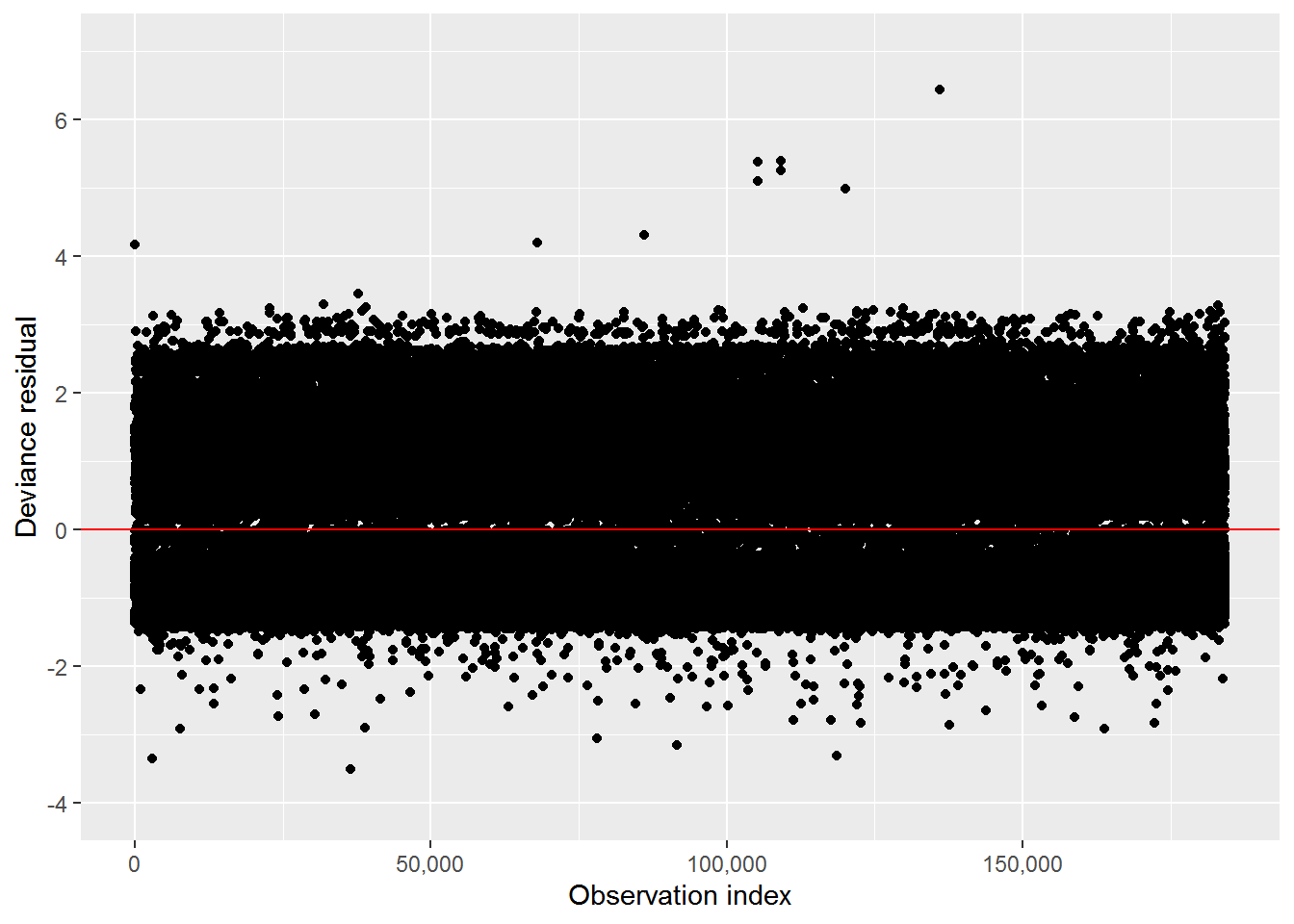
Figure 1: Time-dependent personal vehicle model deviance residuals
Plots of null Cox model Martingale residuals against parking cost, toll cost, household size, origin and destination TAZ parking, and origin and destination TAZ terminal time revealed no drastic deviations from linearity, so no functional forms were changed in the time-dependent model. However, exact linearity did not appear to be achieved for any of these covariates, indicating better functional forms likely exist for the inclusion of these covariates in the model. For this analysis, linearity was deemed “close enough” in the context of time and processing limitations.
Having estimated and validated a Cox proportional hazards model for personal vehicle travel time decay, the estimated survival curve was compared to the sample curve for the “most common set of conditions”. For personal vehicle travel, the most common set of conditions was:
- Parking cost = $0
- Toll cost = $0
- Household size = 4
- Purpose = Non-work
- Origin TAZ parking = $0
- Destination TAZ parking = $0
- Origin TAZ terminal time = 1 minute
- Destination TAZ terminal time = 1 minute
A graphical comparison of a modeled travel time decay curve to the sample travel time decay curve for these attributes is shown in Figure 2. In addition, a plot of difference in model and the sample trip survival probabilities for these attributes is provided in Figure 3.
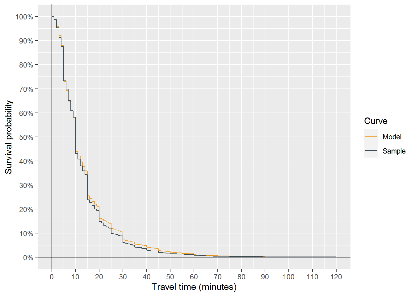
Figure 2: Difference in exampel model and sample survival probabilities for personal vehicle travel
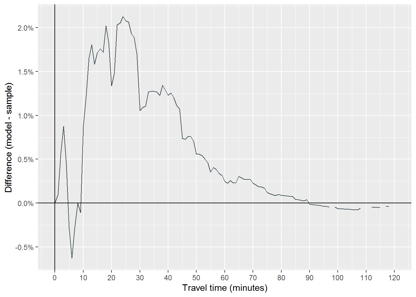
Figure 3: Difference in exampel model and sample survival probabilities for personal vehicle travel
As evidenced in Figures 2 and 3, the model predicted a slower travel time decay than is reflected in the sample, overpredicting survival probability at nearly every point. However, that the maximum absolute error at any time point is just over 3% indicated that the model reflects the sample well.
4.2 NON-MOTORIZED
The model including all candidate covariates showed household size was an insignificant contributor to hazard. When backward selection was used to exclude household size, a statistically valid fit was achieved. The final initial model included only purpose (again, the purpose “home” was used as the reference level for fitting the purpose covariate). The model coefficients are provided in Table 10, while the hazard ratios are provided in Table 11.
| Covariate | ß | SE(ß) | z | Pr(>|z|) |
|---|---|---|---|---|
| Destination TAZ parking | 0.0053 | 0.0007 | 7.6080 | < 0.0001 |
| Destination TAZ terminal time | -0.1714 | 0.0094 | -18.2873 | < 0.0001 |
| Purpose: work | 0.3069 | 0.0235 | 13.0760 | < 0.0001 |
| Purpose: non-work | 0.3908 | 0.0165 | 23.6941 | < 0.0001 |
| Covariate | HR | Inverse HR | 95% CI for HR |
|---|---|---|---|
| Destination TAZ parking | 1.0053 | 0.9947 | [1.0039, 1.0067] |
| Destination TAZ terminal time | 0.8425 | 1.1869 | [0.8272, 0.8581] |
| Purpose: work | 1.3592 | 0.7357 | [1.2981, 1.4232] |
| Purpose: non-work | 1.4782 | 0.6765 | [1.4312, 1.5267] |
Schoenfeld Residuals Tests on the covariates revealed time dependence in the non-work purpose, but not for the work purpose. The results of the test are shown in Table 12. A time-dependent coefficients model was explored as a result of present time dependence
| Covariate | \({\rho}\) | \({\chi^2}\) | p |
|---|---|---|---|
| Destination TAZ parking | 0.0332 | 21.8417 | < 0.0001 |
| Destination TAZ terminal time | 0.0312 | 19.3586 | < 0.0001 |
| Purpose: work | -0.0134 | 3.8630 | 0.0494 |
| Purpose: non-work | -0.0548 | 64.7239 | < 0.0001 |
| Global | 126.6509 | < 0.0001 |
Exploration of scaled Schoenfeld residuals vs. time plots followed by iterative model fitting and re-checking of the proportional hazards assumption resulted in a time-dependent coefficients model with a single break point at 5 minutes. This model featured no time dependence, and thus this model was used going forward. The model coefficients are provided in Table 13, while the hazard ratios are provided in Table 14.
| Covariate | Interval | ß | SE(ß) | z | Pr(>|z|) |
|---|---|---|---|---|---|
| Destination TAZ parking | 0-5 minutes | 0.0024 | 0.0010 | 2.3269 | 0.02 |
| Destination TAZ parking | > 5 minutes | 0.0084 | 0.0009 | 9.0147 | < 0.0001 |
| Destination TAZ terminal time | 0-5 minutes | -0.2198 | 0.0162 | -13.5900 | < 0.0001 |
| Destination TAZ terminal time | > 5 minutes | -0.1465 | 0.0115 | -12.7736 | < 0.0001 |
| Purpose: work | 0-5 minutes | 0.3530 | 0.0371 | 9.5180 | < 0.0001 |
| Purpose: work | > 5 minutes | 0.2881 | 0.0304 | 9.4703 | < 0.0001 |
| Purpose: non-work | 0-5 minutes | 0.5299 | 0.0264 | 20.0958 | < 0.0001 |
| Purpose: non-work | > 5 minutes | 0.2871 | 0.0214 | 13.4093 | < 0.0001 |
| Covariate | Interval | HR | Inverse HR | 95% CI for HR |
|---|---|---|---|---|
| Destination TAZ parking | 0-5 minutes | 1.0024 | 0.9976 | [1.0004, 1.0045] |
| Destination TAZ parking | > 5 minutes | 1.0085 | 0.9916 | [1.0066, 1.0103] |
| Destination TAZ terminal time | 0-5 minutes | 0.8027 | 1.2459 | [0.7776, 0.8285] |
| Destination TAZ terminal time | > 5 minutes | 0.8637 | 1.1578 | [0.8445, 0.8833] |
| Purpose: work | 0-5 minutes | 1.4233 | 0.7026 | [1.3235, 1.5306] |
| Purpose: work | > 5 minutes | 1.3339 | 0.7497 | [1.2567, 1.4159] |
| Purpose: non-work | 0-5 minutes | 1.6988 | 0.5887 | [1.6132, 1.7889] |
| Purpose: non-work | > 5 minutes | 1.3325 | 0.7504 | [1.2778, 1.3897] |
The plot of deviance residuals for the updated, time-dependent model is shown in Figure 4. Though a few potential outliers are observed in the “trip ended later than expected” category (very negative deviance residuals), they are small in number, and individual exploration revealed no grounds on which to exclude any points as outliers.
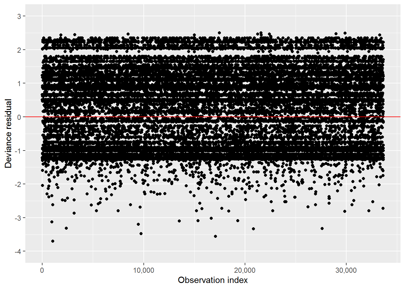
Figure 4: Time dependent non-motorized model deviance residuals
Plots of null Cox model Martingale residuals against destination TAZ parking and destination TAZ terminal time revealed no drastic deviations from linearity, so no functional forms were changed in the time-dependent model. However, like with the personal vehicle model, exact linearity did not appear to be achieved for any of these covariates, indicating better functional forms likely exist for the inclusion of these covariates in the model. For this analysis, linearity was deemed “close enough” in the context of time and processing limitations.
Having estimated and validated a Cox proportional hazards model for non-motorized travel time decay, the estimated survival curve was compared to the sample curve for the “most common set of conditions”. For non-motorized travel, the most common set of conditions was:
• Destination TAZ parking = $0 • Destination TAZ terminal time = 0 minutes • Purpose = Non-work
A graphical comparison of a modeled travel time decay curve to the sample travel time decay curve for these attributes is shown in Figure 5. In addition, a plot of difference in model and the sample trip survival probabilities for these attributes is provided in Figure 6.
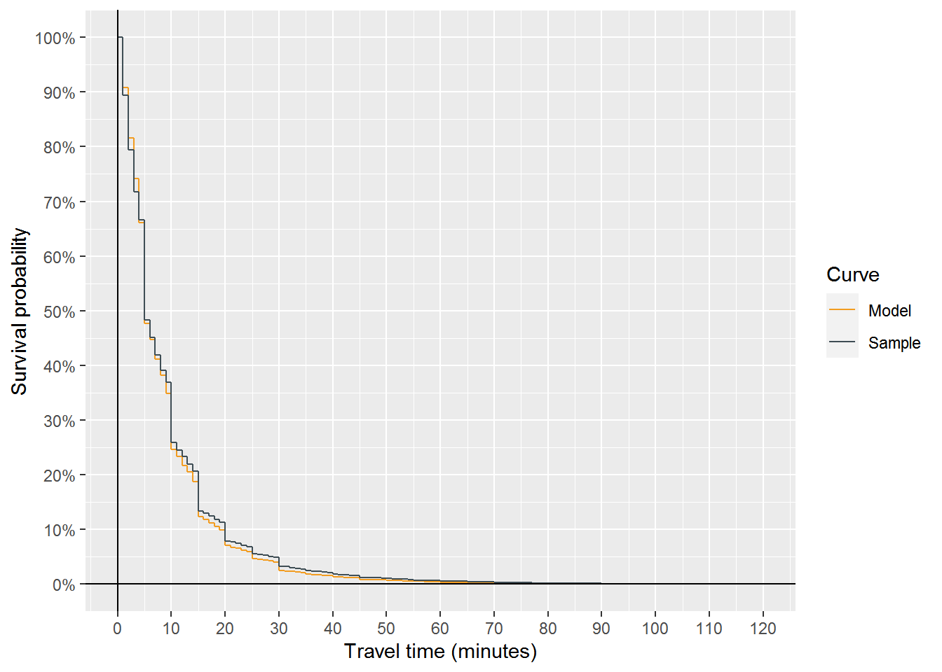
Figure 5: Example comparison of model and sample travel time decay curves for non-motorized travel
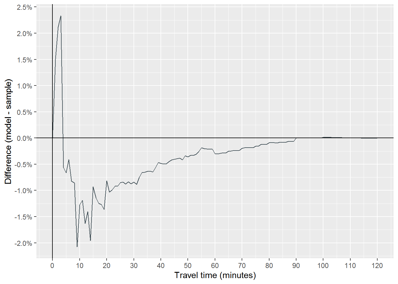
Figure 6: Difference in example model and sample survival probabilities for non-motorized travel
As evidenced in Figures 5 and 6, the model predicted a quicker travel time decay than is reflected in the sample, underpredicting survival probability at most points. However, that the maximum absolute error at any time point is just over 2% indicated that the model reflects the sample well.
5 OPERATIONALIZING THE MODEL
Ultimately, it is hoped that this model would be used to answer the following question: how would a change in policy impact trip making? Answering this question relies on comparing the estimated probability density of survival times under varying conitions, and adjusting for natural de-valuing of longer distance trips.
5.1 DERIVING A DECAY FACTOR
Consider two cases: a null case \(\scriptstyle C_0\) representing the existing conditions, and an alternative case \(\scriptstyle C_A\) representing some sort of change in the travel system (e.g. an increase in toll cost). Define a decay factor \(\scriptstyle D_{t,C_0,C_A}\) Dt,C0,CA as the value of a trip of duration t based on:
- the duration of the trip, t
- the change in conditions from \(\scriptstyle C_0\) to \(\scriptstyle C_A\).
5.1.1 TRIP DURATION COMPONENT
For the trip duration component, we need to tackle the question what proportion of people are willing to travel t minutes? To answer this, consider the population of people traveling more than t minutes under the existing conditions \(\scriptstyle C_0\). Recall that the survival function \(\scriptstyle S(t) = P(T > t)\), so this population is \(\scriptstyle (100·S_{C_0} (t))\)% of all people. The trip duration for people in this set include \(\scriptstyle t+ 1, t+ 2, ..., t_{max}\) (because time is discrete in this analysis). Under equal circumstances, we assume that a person whose trip falls in this set would choose to travel the minimum time of the set if given the choice. In other words, all people traveling longer than t would choose to travel t + 1 if they could. By this logic, \(\scriptstyle S_{C_0} (t)\) is a measure of “willingness to travel t + 1 minutes”: \(\scriptstyle (100·S_{C_0} (t))\)% would travel t + 1 minutes if they could. It follows that \(\scriptstyle S_{C_0} (t-1))\) gives the proportion of people willing to travel t minutes, which answers the initial question.
5.1.2 CHANGE IN CONDITION COMPONENT
For the change in conditions component, we need to tackle the question how does the likelihood of taking a t minute trip change between \(\scriptstyle C_0\) and \(\scriptstyle C_A\) ? To answer this, we can rely on the formulation of survival curves. Consider the following mathematical equivalencies:
\[ \begin{aligned} S(t) &= P(T > t) && \text{(definition of survival function)} \\ &= 1 - P(T \le t) && \text{(probability rules)} \\ &= 1 - F(t) && \text{(definition of cdf)} \\ &= 1 - \int_0^t f(t)dt && \text{(relationship between cdf and pdf)} \\ &= 1 - \sum_0^t f(t) && \text{(equivalency due to discrete nature of } t \text{)} \\ &= 1 - \sum_0^t P(T = t) && \text{(definition of pdf)} \end{aligned} \]
\(\scriptstyle f(t) = P(T = t)\) is the value of interest here, because it defines the likelihood of taking an exactly t minute trip. To understand how f(t) can be calculated from survival probabilities, consider the following:
\[ \begin{aligned} F(t) &= \sum_0^t f(t) \\ \text{Then: } F(0) &= f(0) \\ &= 0 \\ F(1) &= f(0) + f(1) \\ &= F(0) + f(1) \\ &\bf{\implies} \ f(1) = F(1) - F(0) \\ F(2) &= f(0) + f(1) + f(2) \\ &= F(1) + f(2) \\ &\bf{\implies} \ f(2) = F(2) - F(1) \\ F(3) &= f(0) + f(1) + f(2) + f(3) \\ &= F(2) + f(3) \\ &\bf{\implies} \ f(3) = F(3) - F(2) \\ &\vdots \\ F(t) &= f(0) + f(1) + ... + f(t) \\ &= F(t-1) + f(t) \\ &\bf{\implies} f(t) = F(t) - F(t-1) \\ \end{aligned} \]
It then follows that: \[ \begin{aligned} f(t) &= F(t) - F(t-1) \\ &= 1 - S(t) - [1 - S(t-1)] \\ &= 1 - S(t) - 1 + S(t-1) \\ &= S(t-1) - S(t) \end{aligned} \]
So, the likelihood of taking an exactly t minute trip \(\scriptstyle f(t) = S(t − 1) − S(t)\). For our cases \(\scriptstyle C_0\) and \(\scriptstyle C_A\), two unique survival functions \(\scriptstyle S_{C_0}(t)\) and \(\scriptstyle S_{C_A}(t)\) will be estimated, resulting in unique estimates \(\scriptstyle f_{{C_0}}(t)\) and \(\scriptstyle f_{{C_A}}(t)\) for the probability of taking a t minute trip in \(\scriptstyle C_0\) and \(\scriptstyle C_A\) respectively. With these estimates, expected change can be expressed through a density ratio: $ $ represents the factor by which the amount of t minute trips should change with a switch from \(\scriptstyle C_0\) and \(\scriptstyle C_A\), which answers the initial question.
5.1.3 CALCULATING DECAY
Let \(\scriptstyle S_{C_0}(t-1)\) be the proportion of people who would be willing to travel t minutes. Furthermore, let the density ratio $ $ be the factor of expected change associated with trips of t minutes. Then we can calculate a decay factor of the following form:
\[ D_t,C_0,C_A=S_{C_0}(t-1) \bullet \frac{f_{C_A}(t)}{f_{{C_0}(t)}}\]
\(\scriptstyle D_t,C_0,C_A=S_{C_0}(t-1)\) can be interpreted as the proportion of people who would be expected to travel t minutes if given the opportunity in \(\scriptstyle C_A\), assuming the willingness to travel reflected by behavior in \(\scriptstyle C_0\).
5.2 A WALKTHROUGH EXAMPLE
To exemplify this operationalization, imagine that we want to quantify the value of a 15 minute vehicle trip in the context of increasing tolls. The null case \(\scriptstyle C_0\) will assume no tolls. It will be compared to three alternative cases \(\scriptstyle C_{A_i},=1,2,3\) , where i represents a $1, $2, or $3 toll, respectively. All other model variables will be held constant. Table 15 details the covariates in each case.
| Case | Parking cost | Toll cost | Household size | Purpose | Orig. TAZ term. time | Dest. TAZ term. time |
|---|---|---|---|---|---|---|
| C0 | $0 | $0 | 1 | Work | 0 | 0 |
| CA1 | $0 | $1 | 1 | Work | 0 | 0 |
| CA2 | $0 | $2 | 1 | Work | 0 | 0 |
| CA3 | $0 | $3 | 1 | Work | 0 | 0 |
The first step involves calculating the proportion of people willing to travel 15 minutes, or \(\scriptstyle S_{C_0}(14)\). Using the personal vehicle model, we predict a survival curve using the conditions in \(\scriptstyle C_0\), and extract the survival probability at t = 14. We find that \(\scriptstyle S_{C_0}(14)\). A visualization is provided in Figure 7.
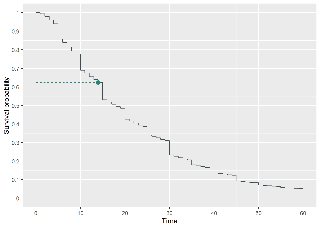
Figure 7: \(S_{C_0}(t)\), with \(S_{C_0}(14)\) highlighted
Next, the probabilities that a trip lasts 15 minutes must be calculated in each alternative case, and then compared to the same probability in the null case. Using the personal vehicle model, we predict survivalcurves for \(\scriptstyle C_{A_1}\), \(\scriptstyle C_{A_2}\), and \(\scriptstyle C_{A_3}\), and calculate \(\scriptstyle f_{CA}(15)\) according to the survival probabilities at t = 14, 15.
We refer back to the null case survival curve to calculate \(\scriptstyle f_{C_0}(15)\) in the same manner. Finally, we take the ratio of each fCAi(15) \(\scriptstyle f_{C_{A_i}}(15)\) to \(\scriptstyle f_{C_{0_i}}(15)\). The results are provided in Table 16. For context, the null and alternative case probability density functions on t ∈ [10, 20] are shown in Figure XXX2.
| Case | Density | Density ratio (to \({C_0}\)) |
|---|---|---|
| C0 | 0.095 | 1.000 |
| CA1 | 0.091 | 0.965 |
| CA2 | 0.062 | 0.655 |
| CA3 | 0.041 | 0.429 |
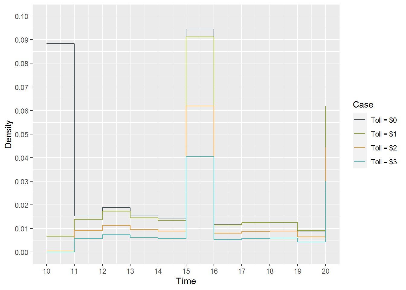
Figure 8: \(f_{C_0}(t)\) and \(f_{C_{A_i}}(t), i=1,2,3\)
Final, the decay factor \(\scriptstyle D_{15,{C_0,C_{A_i}}}=S_{C_0}(14) \bullet \frac{f_{C_A}(15)}{f_{{C_0}(15)}}\) is calculated fro all three \(\scriptstyle C_{A_i}\). The results are provided in Table 17.
| Case | Willingness to travel | Density ratio | Decay factor |
|---|---|---|---|
| CA1 | 0.624 | 0.965 | 0.602 |
| CA2 | 0.624 | 0.655 | 0.409 |
| CA3 | 0.624 | 0.429 | 0.268 |
So, it is learned that, without even considering toll increases, 15 minute trips are de-valued (relative to a less-than-1 minute trip) by a factor of about 0.65 based on time alone. The impact of the toll increase on a 15 minute trip is negligible at $1 (estimated 0.97 times the 15 minute trips), but is notable at $2 and $3 (estimated 0.68 and 0.46 times the 15 minute trips, respectively). It can be concluded that, for the about 65% of travelers willing to take a 15 minute trip, a $1 toll does not drastically alter accessibility, but that a $2 or more toll does.
6 CONCLUSION
A time-dependent Cox proportional hazards model offers an improvement over classical travel time decay modeling methods by allowing for the inclusion of covariate information and quantifying effect sizes associated with these covariates. Furthermore, the use of time-dependent coefficients in these Cox models allows for an interval understanding of covariate effects, which is particularly useful in travel time since trips are often thought of in 5 or 10 minute intervals. The Cox models fit in this analysis indicate that, depending on the mode of choice, trip purpose, trip cost, and household size may all be significant contributors to trip hazard rate and, consequently, trip survival time. These covariates represent a suite of information that should be readily available for use of these modeling in a predictive or simulative context.
Future models should seek to explore additional relevant covariate information (such as terminal time) and/or potential interactions between covariates. They also may seek the following modeling improvements, which were not addressed in this analysis due to processing and time constraints.
- Use of a smoothed function for time-dependent coefficients, as opposed to a step function: Rather than estimating coefficients in discrete time intervals, coefficients could be estimated using a smoothed function of time. For example, in the case of monotonically decreasing effect size with time, a linear function could be valid. This could improve accuracy in estimating effect sizes
- Estimation of proper functional form for continuous covariates: Rather than assuming a basic linear form for continuous covariates, more representative functional forms could be estimated using smoothing techniques, for example. This would improve understanding of the relationship between the covariates and hazard, as well as likely improve predictive accuracy.